
ML concepts : k-means cluster and TF-IDF in Robotics
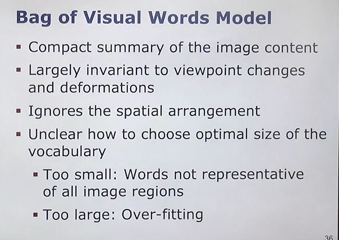
Finding similar images in a database has many applications in robotics, computer vision, and other fields. The basic idea is to find a similar image in the database for a given query image. A popular technique used for this is Bag of Visual Words (BoVW), where images are not stored as they are but as histograms of image features, called visual words. The search image is first converted into a histogram of visual words and then matched with the stored image histograms.
Bag of Visual words
The term "Bag of Visual Words" (BoVW) is similar to technique used in text mining. In text mining, documents are represented as bags of words — essentially histograms of word occurrences. This technique helps find similar documents or categorize them based on word frequency distributions.
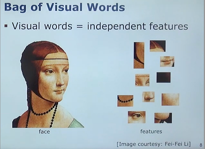
In a similar way, BoVW applies this concept to images. Instead of storing full images, BoVW breaks down images into small patches or features, treating these patches as "visual words."(check the image above). A dictionary of these visual words is created, much like a dictionary of terms in a language, which helps in categorizing and comparing images.
Decomposition
- Image: An image is broken down into small regions or features (visual words). (ref image above)
Representation
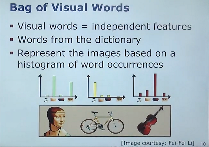
- Feature: These features are converted into a histogram, representing the frequency of each visual word in the image.
Comparison
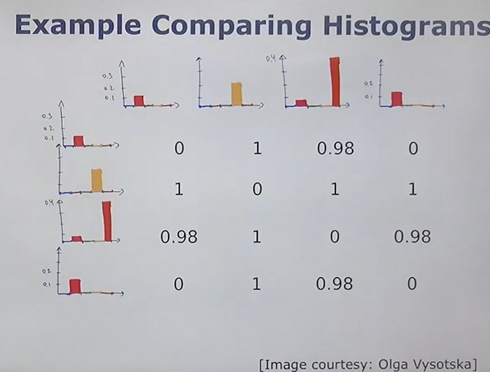
- Comparison: When searching for similar images, the query image is converted into a histogram of visual words. This histogram is then compared to the histograms of images in the database.
Matching
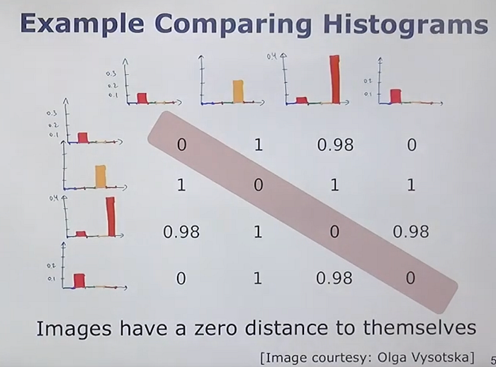
- Matching: Images with similar histograms (i.e., similar distributions of visual words) are considered similar.
This method allows for efficient image search and categorization by focusing on feature occurrence patterns rather than storing and comparing raw image data.
Visual Dictionary
Pixel information is converted into visual words using features and feature descriptors, such as SIFT features. This involves breaking down an image into independent features, which are then used to represent the image. These features, illustrated as local patches, are easier to visualize.
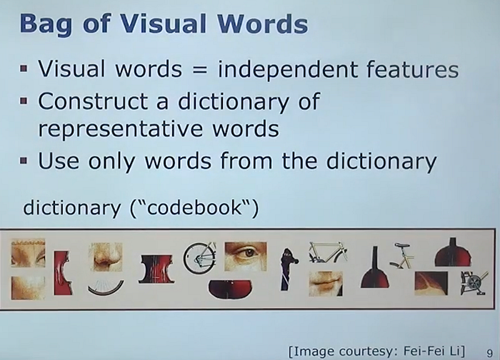
To effectively describe images, a visual dictionary (or codebook) is needed, similar to the Oxford English Dictionary for words. This dictionary defines the allowed visual words (features) for image representation. Various parts of images, like faces, bikes, and musical instruments, contribute to this dictionary, providing wide coverage for different images.
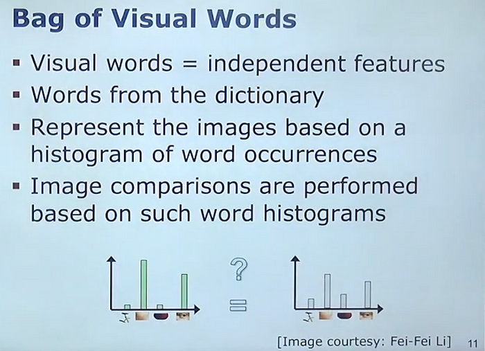
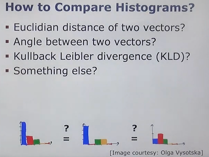
When processing images, histograms are created to show the frequency of each visual word. The BoVW approach compares these histograms rather than the raw images. By evaluating the distribution of visual words using a distance metric or similarity measure, the system determines if two images are similar. This method allows for efficient image search by focusing on feature distributions instead of complete image information.
How it works under the hood?
Image to histogram
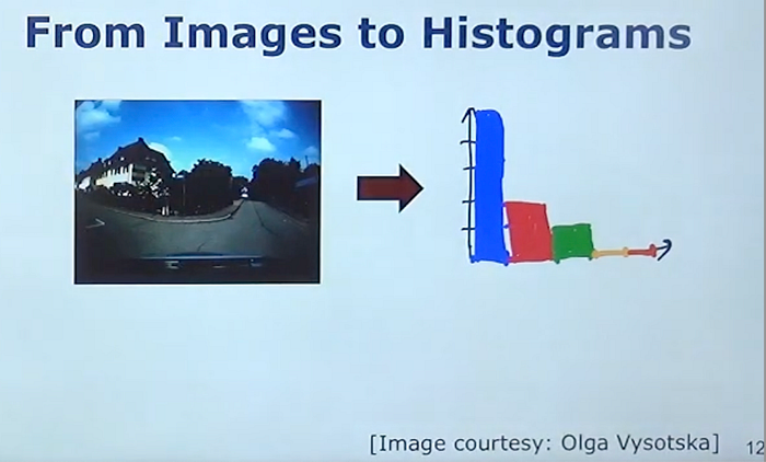
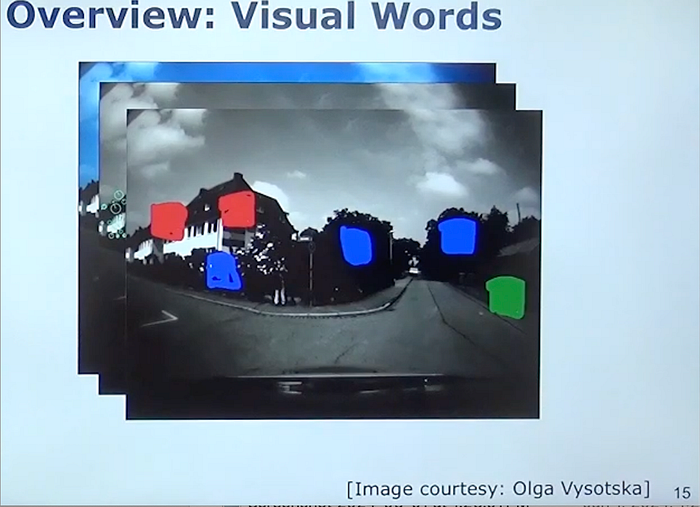
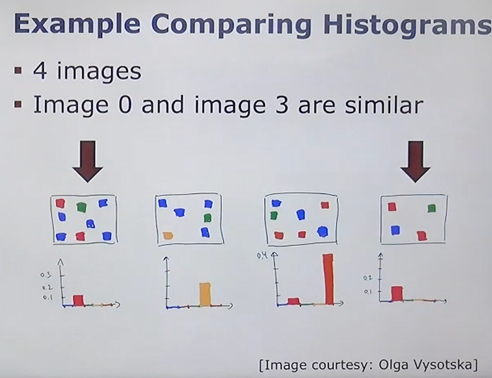
Images are converted into histograms of feature occurrences. For example, imagine an image recorded from a car-mounted camera while driving around a city to solve visual place recognition tasks. The goal is to be able to recognize the same locations under different conditions by comparing current camera images to a database of previously taken images.
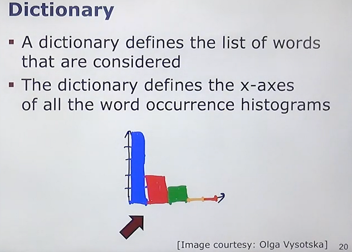
To achieve this using the Bag of Words (BoW) approach, the first step is to transform an image into a histogram of visual words. The x-axis of the histogram represents the visual words (shown as different colors for illustration), and the y-axis represents their counts. For instance, a blue visual word might appear five times, a red one twice, a green one once, and others not at all. This transformation from image to histogram is essential for the BoW method.
Visual Words
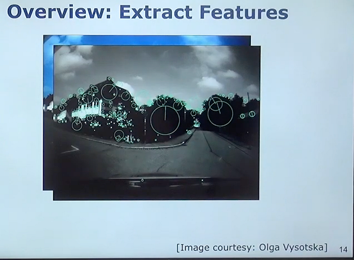
To turn images into histograms of feature occurrences, we start with an input image and extract visual features using a method such as SIFT (Scale-Invariant Feature Transform). SIFT identifies key points in the image and describes them based on their local neighborhood. Each key point is represented by a circle whose center is the key point location, the line indicates orientation, and the circle size indicates the detection scale.
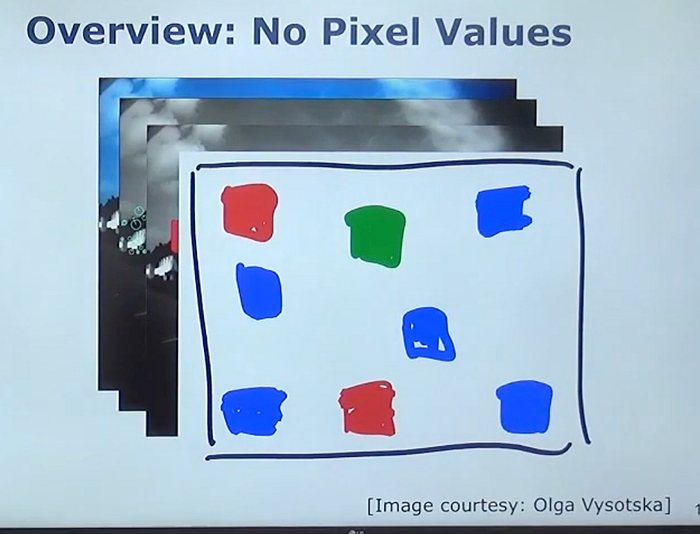
Once the SIFT features are extracted, they must be reduced to visual words. This process involves using a predefined dictionary of visual words. Each visual word represents a set of similar features. The extracted features are assigned to the closest word in the dictionary, and if a feature is too distant from any word, it may be ignored. For illustration, features could be mapped to colored boxes (e.g., blue, green, red), representing different visual words.

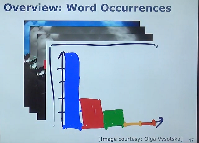
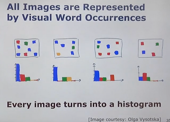
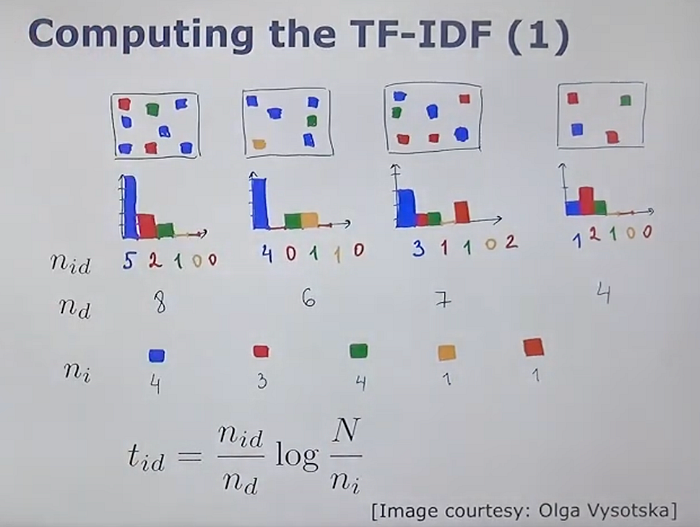
After mapping the features to visual words, the image itself can be disregarded. We then count the occurrences of each visual word in the image, forming a histogram. For example, if the blue visual word appears five times, the red one twice, and the green one once, the histogram might look like 5, 2, 1, 0, 0. This histogram can be expressed as a vector, and every image can be converted into such a histogram of visual words.
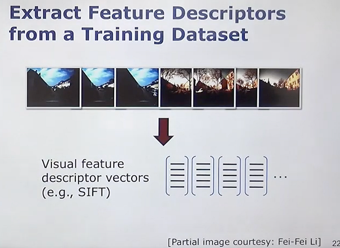
To create the dictionary of visual words, we need a feature descriptor (e.g., SIFT) and a method to define the visual words. The dictionary must be fixed, defining which visual words are allowed and their order in the histogram. Typically, the dictionary is learned from a large and diverse dataset, which should be representative of the types of images the system will later encounter. This dictionary remains constant once learned.
The process of learning the dictionary involves taking a large training dataset, extracting visual features (e.g., SIFT features), and then clustering these features to define the visual words. This results in a fixed set of visual words, each representing a cluster of similar features.
Once the dictionary is established, we can convert any new image into a histogram of visual words by extracting features, mapping them to the closest visual words in the dictionary, and counting their occurrences. This allows us to represent images as vectors of feature occurrences, facilitating tasks such as image comparison and recognition based on the distribution of visual words.

Data Points:
Data points are in some high-dimensional space. In this high-dimensional feature space, all these vectors are just kind of points in this 128-dimensional space. Since it's difficult to visualize a 128-dimensional space , but eaiser to visulize in visualize in 2D.
These are data points stored in this high-dimensional space. Now, what we want to do is group similar features together so they will later form one visual word. Take data points that are close together.

These features provide a description of the local surrounding of the key point, like a distribution of gradients. This means we have data points representing image regions with a similar distribution of gradients. We can turn this distribution into a visual word.
Take the mean of these three data points to make one visual word. We do the same for other groups of data points, illustrated here by color. All the red data points combine to form one red visual word, and the same holds for the green ones.
This grouping of similar descriptors uses a clustering algorithm, which clusters our data points in an unsupervised way. This gives us clusters of feature descriptors in this high-dimensional feature space, and we can find representatives for these clusters. This can be one feature from the subset or, typically, a mean feature descriptor vector computed over those data points.
By running a clustering algorithm, all those data points will turn into a blue word, a yellow word, a green word, and so on. This is a standard clustering approach. The first thing we typically try is something like k-means. Remember, the k-means algorithm is a standard approach.
For clustering using k-means algorithm. A brief introduction to k-means:
The k-means algorithm partitions data (in this case, feature descriptors) into k clusters. We specify k, for example, k = 1,000, to generate 1,000 clusters from the data set and return 1,000 centroids (the centers of these clusters). Each centroid is the mean of the feature descriptors within its cluster, forming one visual word.
Key Steps of the k-means Algorithm:
- Initialization: Randomly sample k data points as initial centroids.
- Assignment: Assign each data point to the closest centroid, minimizing the squared distance between data points and centroids.
- Update: Recompute each centroid as the mean of the data points assigned to it.
This process repeats until convergence, where data assignments and centroid locations stabilize.
In the context of learning our dictionary for the bag-of-visual-words approach, we partition the feature space into k groups. For example, we could group 1 million features into 10,000 clusters, reducing 1 million data points to 10,000 centroids. Each centroid represents a visual word in our dictionary.
During feature detection in an image, we assign each feature to the closest centroid in our dictionary, thus generating visual words that describe the image content.
The k-means algorithm continues to adjust the centroids and assignments to minimize the squared distances between features and centroids, ensuring an optimal grouping of similar features into visual words
Similarity Queries
We use our database to store the TF-IDF weighted histograms for all images. When we want to find a similar image, we follow these steps:
- Feature Extraction: Extract features from the query image using the SIFT detector.
- Visual Word Assignment: Assign each detected feature to a visual word. If a feature is very far from any visual word, we ignore it.
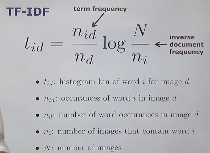
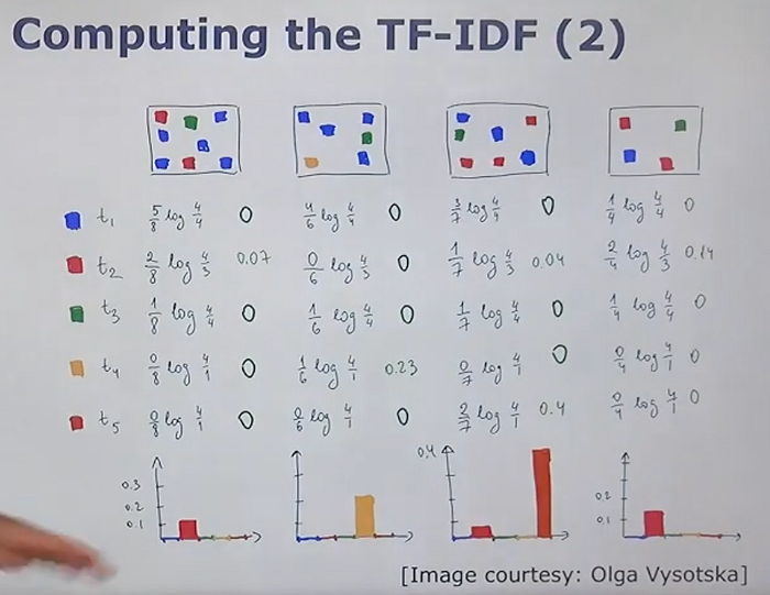
- TF-IDF Weighting: Compute the TF-IDF weighting for the histogram of the query image.
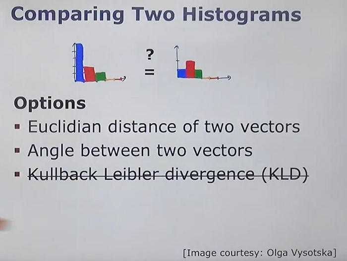
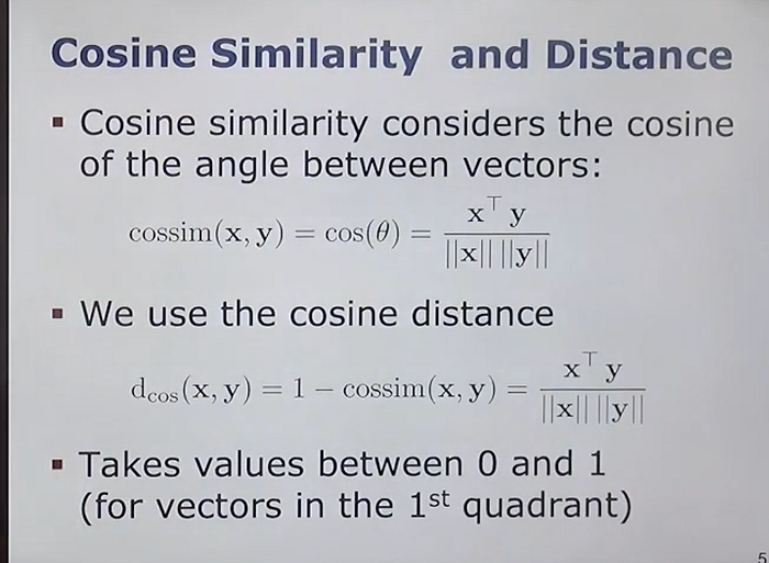
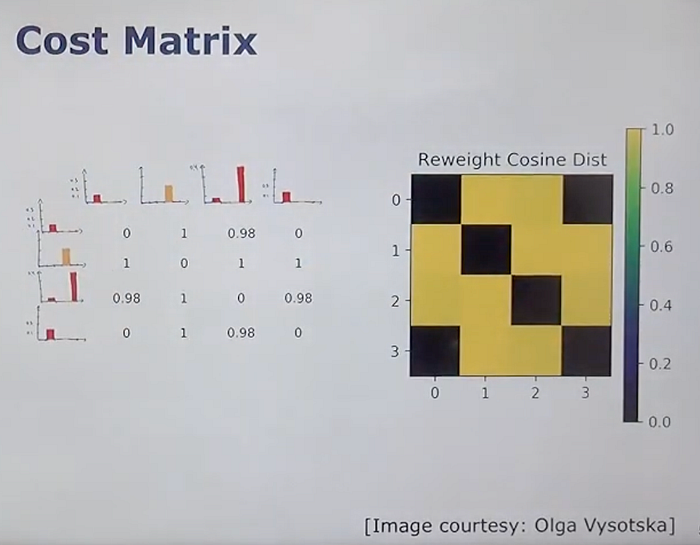
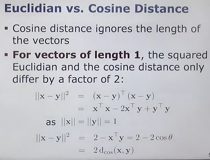
- Cosine Distance Comparison: Compare the TF-IDF weighted histogram of the query image with the histograms of all images in the database using cosine distance.
- Retrieve Similar Images: Return the top n most similar histograms (or corresponding images) from the database.
This process helps us identify the most similar images based on the features and their importance as determined by TF-IDF weighting.
Summary of Bag of Words Approach
The Bag of Words approach is a compact way to describe images and perform similarity queries, frequently used in computer vision and robotics for tasks like 3D reconstruction, localization, and visual place recognition.
- Visual Words Dictionary: Images are described using a dictionary of visual words, counting how often each visual word appears.
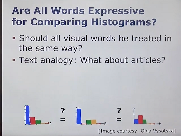
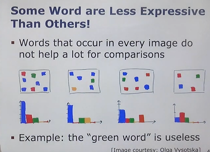
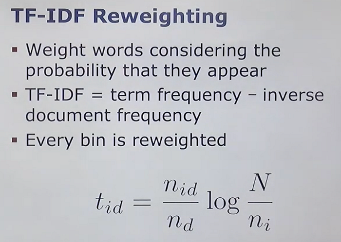
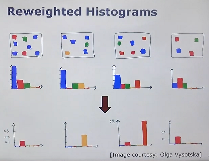
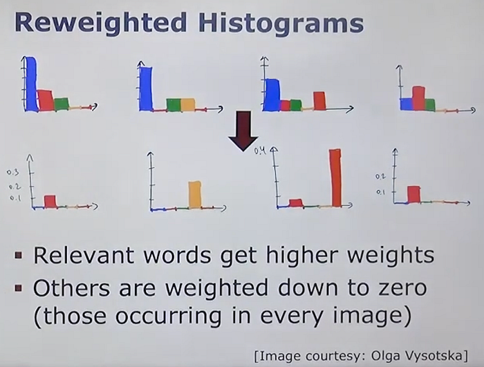
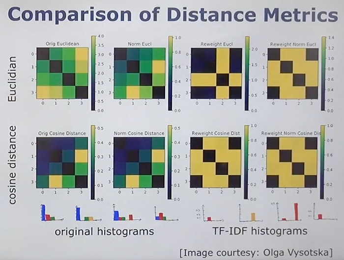
- TF-IDF Reweighting: Enhances the importance of more expressive words for comparison while down-weighting less expressive ones to zero if necessary.
- Cosine Distance: The similarity between images is computed based on the cosine distance of their TF-IDF weighted histograms.
This method is crucial for various applications, including finding loop closure candidates in SLAM or performing initial metric localization in robotics.
