Blog

from paper

Brief SLAM understanding

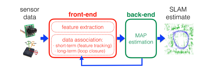
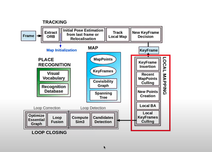
Structure of a typical SLAM System. Back-end infor-

mation can sometimes be fed back into the front-end to assist in data

SLAM, describes a solution to the problem of placing a robot at an unknown location and having it to build a map of its environment while localizing itself inside the map. The vehicle should be able to estimate
its trajectory and the location of the landmarks in real-time, without the need for any a priori knowledge about the area inside which it is inserted.
A SLAM system includes two main components: the front-end and the back-end.

The first is responsible for getting the sensor data and computing it into information that can be used for estimation, as well as data association tasks such as feature tracking and loop closure.

The second component is responsible for performing inference on the information captured by the front end. A typical configuration can be seen in Figure above. It is worth noting that, in this Figure, MAP estimation means Maximum a Posteriori estimation, a Bayesian method used to calculate the estimate of an unknown quantity, based on maximizing the posterior probability in Bayes’ theorem.

A SLAM process can be divided into the following steps

1. Landmark Extraction

This consists in collecting and registering features in the environment that are easily re-observed and distinguished (landmarks). Such features can include corners, blobs, or even edges, and can be represented by pointclouds, when the input sensor is a LiDAR, or images
when the input sensor is a camera. In the latest case, sometimes distortion correction is also needed to be able to correctly extract these features.

2. Data Association

This step takes the features extracted, as well as their estimated locations, and tries to match them (if it is the case) with the same features extracted in the past, or adds new features, in order to build the map. Common problems that arise in this step include as failure to observe the same landmarks in every time step, wrong identification of a landmark, or the
wrong association of landmarks between time steps. To be able to minimize them, more computing power is needed, which means more time, so this process becomes a tradeoff between map accuracy and processing time.

3. Pose and Map Update

Here, the process uses filters such as the Extended Kalman Filter (EKF) or the Particle Filter to estimate the pose of the mobile robot in relation to the map that has being built, updating the information according to what is being computed.

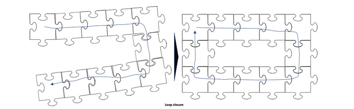
4. Loop closure

As the system continues to get new information on its environment, it might recognize that it is at a point that has been previously visited. This is where loop closure comes into action, completing the map and correcting accumulated errors. A graphical explanation of how loop closure can be useful is shown in Figure below

loop closure

Features-based methods consist in detecting features in the captured image and comparing it to previous frames to detect if the robot has already been in that position. This method, even though it eliminates the accumulated error that comes with geometry- based methods, can become very heavy, since there is a need to compare each new frame with every previous one captured.

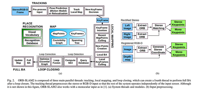
With this background in place, let’s discuss ORB-SLAM2 is a Visual SLAM (Simultaneous Localization and Mapping) system designed for monocular, stereo, and RGB-D cameras. It can accurately track camera motion and reconstruct the 3D environment. Some of the essential features include loop closure, relocalization, and the use of ORB (Oriented FAST and Rotated BRIEF) features for efficient and reliable map creation.

ORB (Oriented FAST and Rotated BRIEF) is a method used in computer vision to describe and match important points, like corners or edges, in images. It helps machines understand and track these points as they move around, which is useful for tasks like navigation or building 3D maps of spaces.

In AR/VR applications, ORB-SLAM2 enhances user experiences by providing precise environment mapping and tracking, crucial for overlaying virtual objects in real-world settings and ensuring seamless, immersive interactions in augmented and virtual environments.

In this writing we will go through the implementation details of orb-slam2.

from paper

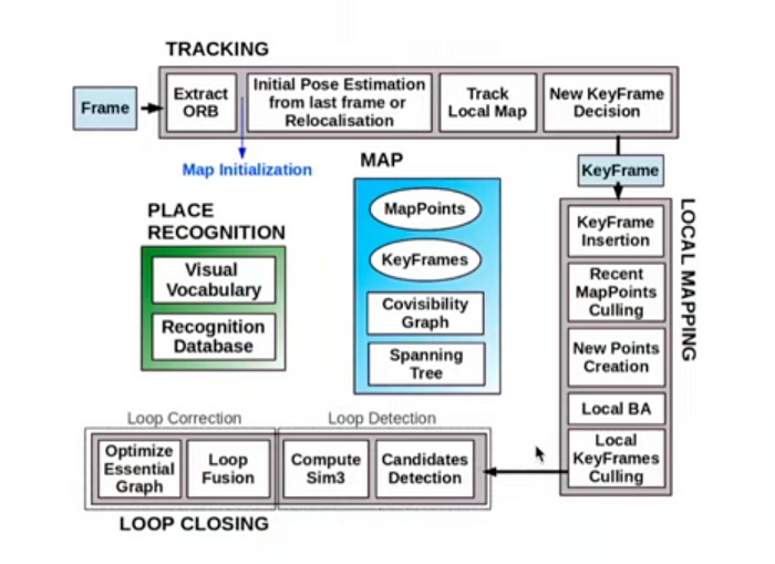
General data structure used in ORB-SLAM2.

Data Structure

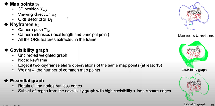
image taken from paper

map point

3D position

Viewing direction vector n_i

A map point data structure is a fundamental element used in mapping and localization algorithms, particularly in visual SLAM (Simultaneous Localization and Mapping). Map points represent 3D locations in the environment relative to the camera, and they are used to build a map of the surroundings as the camera moves through the space. Each map point typically contains information about its position, appearance, and possibly other attributes depending on the specific SLAM algorithm being used.

Key aspects of a map point data structure:

3D Position: The primary aspect of a map point is its 3D position in the world coordinate system. This position is usually represented by a vector (x, y, z) relative to a reference frame.

Appearance Information: Map points store appearance information, such as descriptors or feature vectors extracted from the images captured by the camera. These descriptors help in matching map points across different frames and in performing loop closure, where previously visited areas are recognized.

Observations: Map points are associated with observations or projections in the camera frames where they are visible. These observations consist of pixel coordinates (u, v) and possibly depth information if available.

Association with Keyframes: Map points are often associated with keyframes (reference frames) in the SLAM system. Keyframes contain information about the camera pose and are used to establish the spatial relationships between map points and the camera trajectory.

Overall, the map point data structure is essential for representing the 3D structure of the environment and enabling accurate localization and mapping in SLAM systems. The efficiency and robustness of the SLAM algorithm heavily depend on the quality and management of map points.

The black and the red points are they map points. The blue are the keyframes.

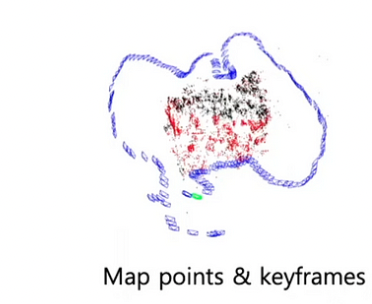
keyframes: subset of general frames. It has the distinctiveness of

Camera Pose : rotation and translation vectors

camera intrinsics (focal length + principal point)

all the ORB features extracted in the frame

In ORB-SLAM2, keyframes are frames of an image or video sequence that are selected based on certain criteria to serve as reference frames for localization and mapping. Keyframes play a crucial role in visual SLAM (Simultaneous Localization and Mapping) systems like ORB-SLAM2, which aim to estimate the camera pose and build a map of the environment concurrently.

Key aspects of keyframes in ORB-SLAM2:

Selection Criteria: Keyframes are typically selected based on factors like motion, scene complexity, or temporal separation. For example, a new keyframe may be chosen if the camera has moved significantly from the previous keyframe, if there’s a notable change in the scene, or if a certain amount of time has passed.

Feature Extraction: Keyframes are used for feature extraction and matching. ORB-SLAM2 uses the Oriented FAST and Rotated BRIEF (ORB) feature detector and descriptor to extract distinctive features from keyframes.

Map Initialization: Keyframes are essential for initializing the map. They provide initial visual information about the environment and help in establishing the relative positions of features in the scene.

Localization: During the SLAM process, keyframes are used for camera localization. The system matches features between the current frame and keyframes to estimate the camera pose relative to those keyframes.

Covisibility graph

The green is the covisibility graph

The green area is thick because it has many edges.

Nodes: are the keyframes

Edges: 2 keyframes sharing observations of same map points (15 at least)

weight(theta): number of common map points

Essential graph

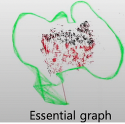
Retains all the nodes

Less number of edges. Subset of edges with high covisibility + loop closure edges.

Loop Closure: Keyframes are also crucial for loop closure detection, where the system identifies previously visited areas by recognizing similarities between the current frame and keyframes. This helps in correcting drift errors and improving the overall accuracy of the SLAM system.

Overall, keyframes act as landmarks in the SLAM process, providing reference points for mapping, localization, and loop closure, thereby improving the robustness and accuracy of the SLAM system like ORB-SLAM2.

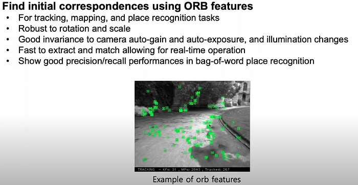
The features are corners, edges or boundaries.

Let’s consider the monocular camera example from ORB-SLAM2 for better understanding of the code.

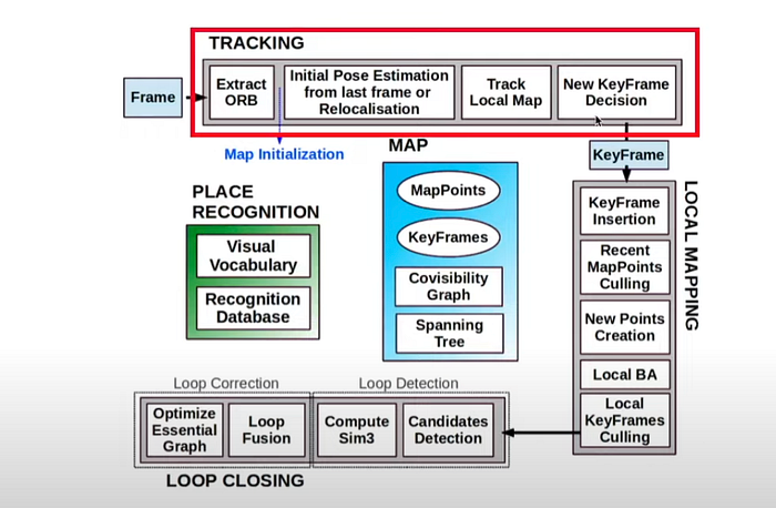
Tracking

Real-Time Pose Estimation: Tracking continuously estimates the camera’s pose relative to the current map. This is done by detecting and matching ORB (Oriented FAST and Rotated BRIEF) features between consecutive frames and computing the transformation between them.

Maintaining Frame-to-Frame Continuity: By ensuring that the camera’s position and orientation are known at all times, tracking maintains continuity in the sequence of images. This is crucial for applications that rely on smooth and consistent visual data, such as augmented reality (AR) and virtual reality (VR).

Ensuring Visual Odometry: Tracking provides a form of visual odometry by calculating the relative motion of the camera between frames. This helps in understanding the camera’s movement and updating its trajectory over time.

Handling Occlusions and Fast Movements: Tracking includes mechanisms to handle challenging situations, such as occlusions or rapid movements, by using predictive models and re-localization techniques. This ensures robustness in various dynamic environments.

Facilitating Keyframe Insertion: Tracking decides when to insert new keyframes into the map. Keyframes are critical for map expansion and long-term stability of the SLAM system, but this decision is primarily made based on tracking performance and the need for new viewpoints.

Tracking

Refer: ORB-SLAM2 Example/Monocular/mono_tum.cc#main

Calls stack: SLAM created
ORB_SLAM2::System SLAM(argv[1],argv[2],ORB_SLAM2::System::MONOCULAR,true);

Refer: System.cc#System

System has Threads for Tracker, LocalMapper and LoopCloser

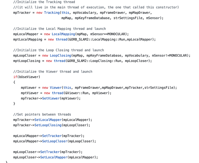
Threads for Tracker, LocalMapper and LoopCloser

load the images and then call TrackMonocular on SLAM class

refer Examples/Monocular/mono_tum.cc#main

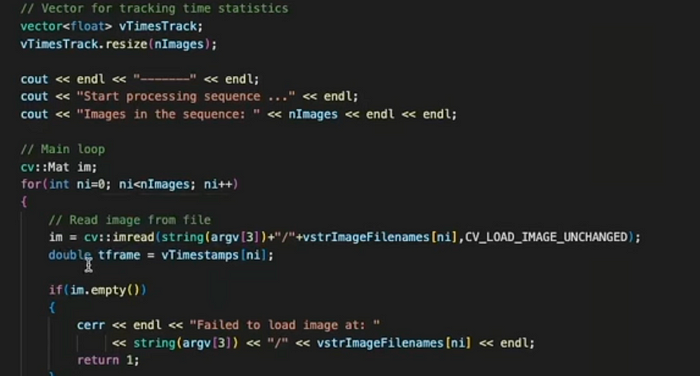
read image frames from dataset

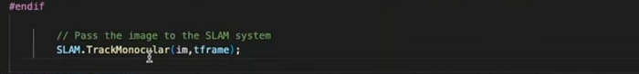
pass the images to the SLAM system here — it’s the tracking part of 2 consecutive image frames

System.cc#TracMonocular

a) ORB Extractors

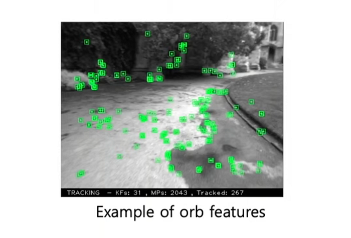
the features are edge

refer Frame.cc#Extractor

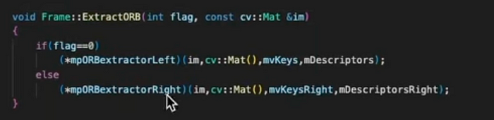
ORB extractor

Refer: Tracking.cc

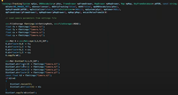
camera parameters — focal length, principal points, distorsion factors

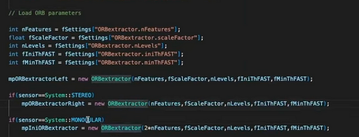
ORB parameters

ORB Extractors are created

orb extractor

b) Map Initialization

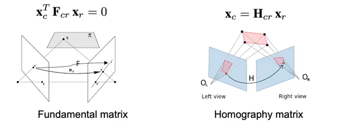
if the scenes are more general — then fundamental matrix is a good model

If the scene includes planner structure — then homographic model is appropriate.

one of these model is selected the map based on the score of the symmetric transfer distance.

The Map Initialization is important, after the model is selected.

refer Frame.cc#Extractor

ORB extractor

Calculate the symmetric transfer distance for 2 models

After selecting the proper model for the scene, we now know the relative transformation between 2 views. This allows us to create 3D model , now we know the model, initialize the map.

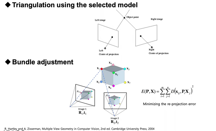
you calculate the relative motion between frames 2 views.

Triangulation — create 3D Map by triangualtion by using the selected model.

then Refine the camera pose and map point using bundle adustment non-linear optimization model. difference between projected point and corresponding point for the image scene.

Map initialization with generic scene

example:

1. extract the ORB features from the general scene the and then initialize the map structure by selecting the right model and then initialize the map.
   

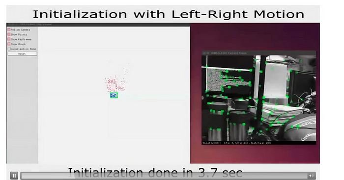
the black and the red dots

The green box is the initialized map.

c) Initial pose estimation

There are 2 cases, when the tracking is successful and when when it fails.

Case I

if the tracking is successful for the last frame, then we are going to estimate the initial pose of the current frame by using

Then refine the camera pose using the motion only using bundle adjustment.

then the delete the right before velocity value will be enough to estimate the camera pose initially. Can refibe camera pose by using BA.

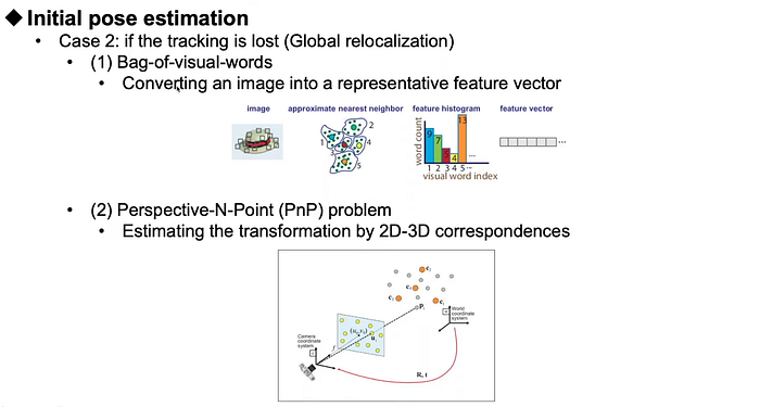
Case II

1. if tracking fails, then use the bag-of-visual-words to detect loop closure. First convert image frame into representative feature vector. Second compare the image frame with all the frames till now saved in the database. We can find similar scene for loop closer .. go to the geometric verification step using

2. PnP — where the camera is located. given the 2D and 3D correspondences in the scene, we can estimate the correct couter pose of the scene and find the the tracking we can record the counter pose where it is now.

d) Track local map

Exceptions to have compact map representation:

1. Map point is outside the image boundary — discard
2. Is the viewing direction of the map point has a big difference with the camera viewing point then — discard
3. Map point is outside of the depth interval, i.e, far away or very close to the camera then remove it.
4. Survived map points are matched by ORB descriptors for later tracking.

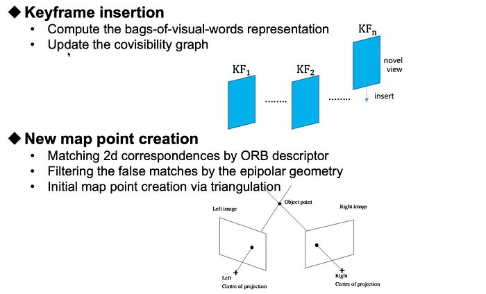
e) New keyframe Decision

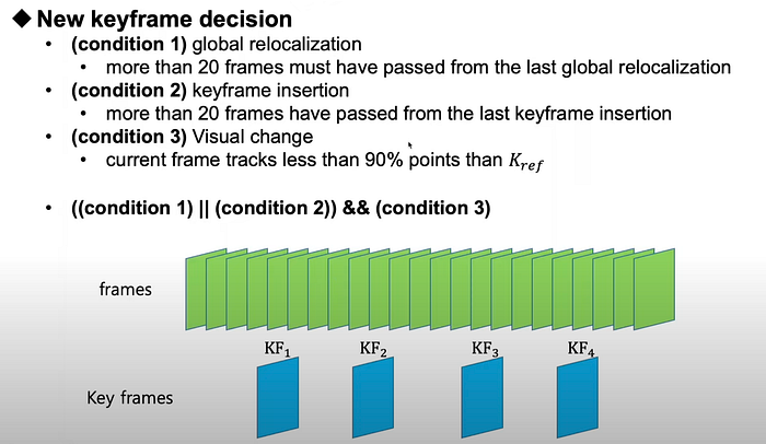
new keyframes conditions

Based on the conditions listed, in this step distinctive frames are selected different from general frame (green). Subset of general frames (green) are the keyframes(blue).

So the outcome of this step is the keyframe.

Local Mapping

a) Compute the bags-of-visual-words representation of the new keyframes as described earlier, this will be used for relocalization. New keyframes are inserted into the covisibility graph and added to the graph structure.

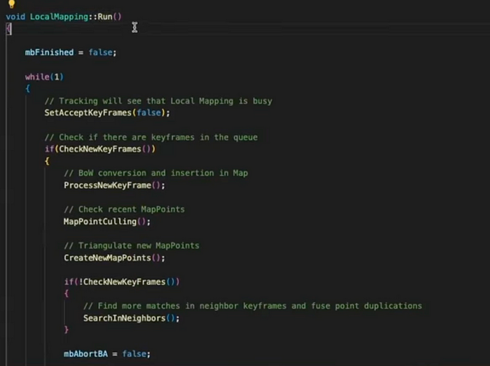
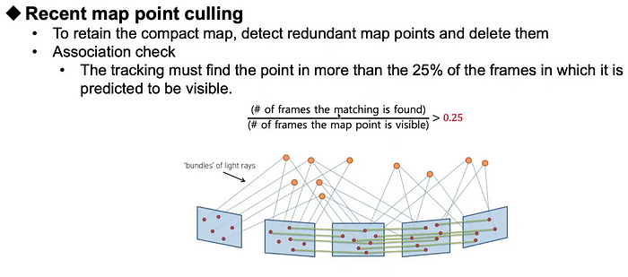
b) compact map — reducndacy check. culling >25%

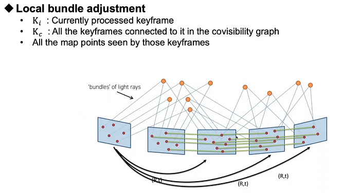
c) After local map is create, local BA is triggered.

d) 

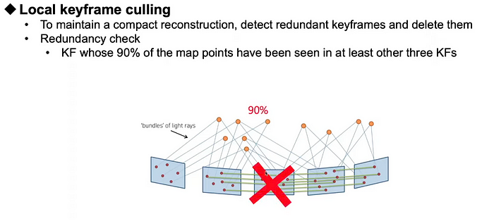
redundancy check

Loop Closing

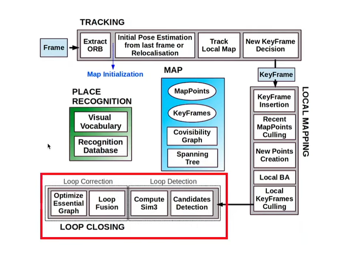
loop closing

LoopClosing.cc#run

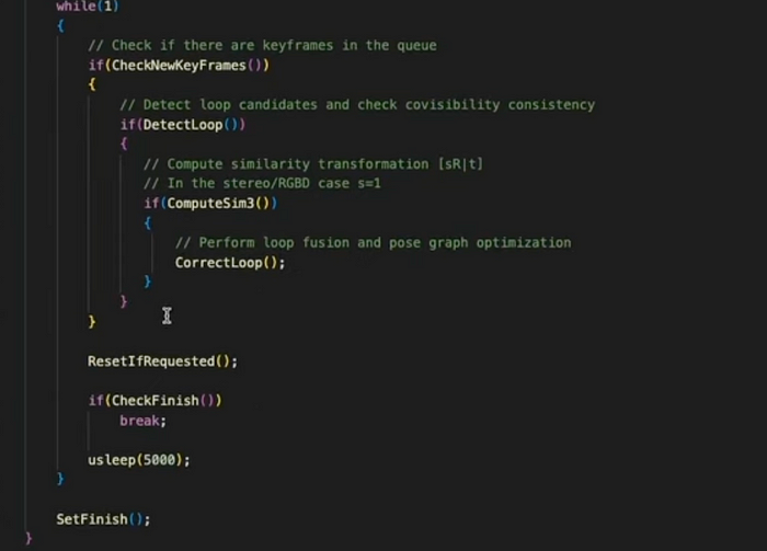
1. loop detection

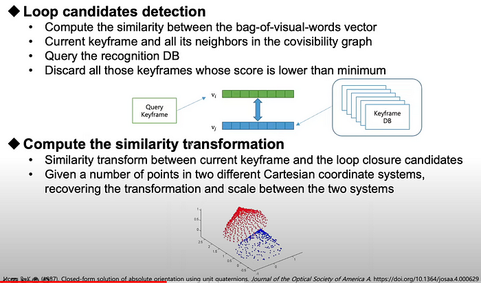
similarity score of the bag of visibility words, in the keyframe db from 1st to last kf, if 2 keyframes are similar — loop closer.

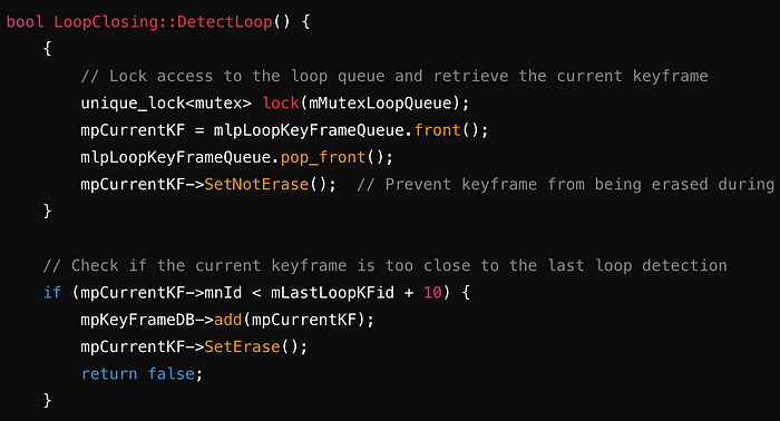
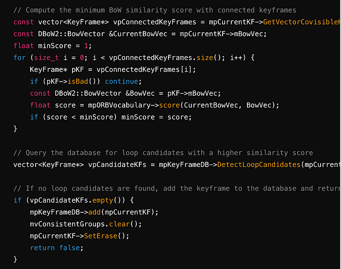
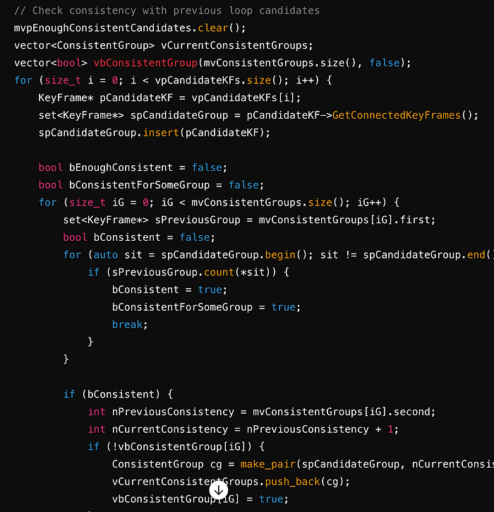
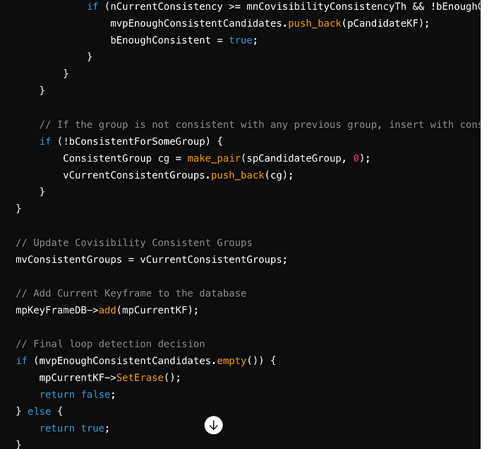
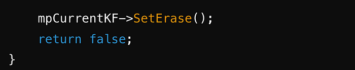
LoopClosing.cc#bool LoopClosing::DetectLoop()

The DetectLoop function in ORB-SLAM2 detects loop closures by evaluating the similarity of the current keyframe with previous keyframes using a Bag of Words (BoW) representation. It ensures that detected loop candidates are consistent with previously detected candidates before confirming a loop closure. This process helps in maintaining the accuracy and robustness of the SLAM system by correcting accumulated drift through loop closures.

loop closer: geometric verification part

BA: refine counterpose in one iteration

2. loop correction

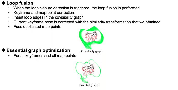
Essential graph optimization:

// Optimize graph

optimizer.cc#Optimizer::OptimizeEssentialGraph(Map* pMap, KeyFrame* pLoopKF, KeyFrame* pCurKF,
const LoopClosing::KeyFrameAndPose &NonCorrectedSim3,
const LoopClosing::KeyFrameAndPose &CorrectedSim3,
const map<KeyFrame *, set<KeyFrame *> > &LoopConnections, const bool &bFixScale)

1. Setup Optimizer
   ├─ Initialize optimizer and solver
   └─ Configure solver parameters
2. Initialize Data Structures
   ├─ Retrieve keyframes and mappoints from the map
   └─ Initialize vectors for transformations and vertices
3. Set KeyFrame Vertices
   ├─ Loop through keyframes
   │ ├─ Create vertex for each keyframe
   │ ├─ Initialize vertex with corrected or non-corrected pose
   │ └─ Fix loop keyframe if necessary
   └─ Add vertices to the optimizer
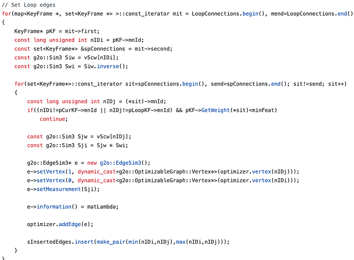
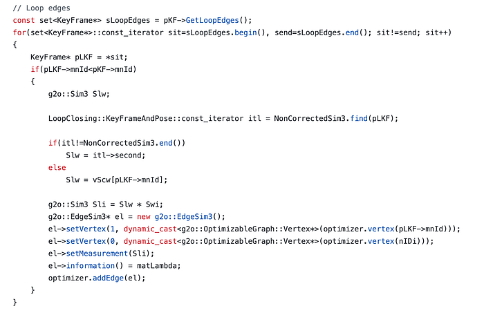
4. Set Loop Edges
   ├─ Loop through loop connections
   │ ├─ For each connection, compute relative Sim3 transformation
   │ └─ Create and add edge to the optimizer
   └─ Store inserted edges to avoid duplicates

1. Setup Optimizer:

A g2o::SparseOptimizer object is created to manage the optimization process.

A linear solver using Eigen is set up and passed to a block solver.

The Levenberg-Marquardt algorithm is selected as the optimization method.

2. Initialize Data Structures:

All keyframes (vpKFs) and mappoints (vpMPs) from the map are retrieved.

Maximum keyframe ID (nMaxKFid) is used to size the transformation and vertex vectors.

4. Set KeyFrame Vertices:

Iterate through each keyframe and create a g2o::VertexSim3Expmap vertex.

Set the initial estimate for the vertex using corrected poses if available, otherwise use non-corrected poses.

Fix the vertex corresponding to the loop keyframe to anchor the optimization.

5. Set Loop Edges:

For each keyframe in the loop connections, compute the relative Sim3 transformation between connected keyframes.

Create edges (g2o::EdgeSim3) representing these transformations and add them to the optimizer.

Store edges to avoid adding duplicates.

6. Set Normal Edges:

Add edges representing parent-child relationships (spanning tree) and other covisible keyframes.

Use non-corrected poses to compute initial transformations and add edges to the optimizer.

7. Optimize:

Initialize the optimization process.

Run the optimizer for 20 iterations to refine keyframe poses.

8. Update KeyFrame Poses:

After optimization, update each keyframe’s pose using the optimized Sim3 transformation.

Convert Sim3 to SE3 and set the pose for each keyframe.

9. Correct MapPoints:

Transform each mappoint’s position based on the optimized pose of its reference keyframe.

Update mappoint positions and normals accordingly to reflect the corrected poses.

This process ensures that the entire map structure is globally consistent after detecting and closing loops, improving the accuracy and robustness of the SLAM system.

After optimizing the essential graph, the global BA is performed in a separate thread as it’s a time comsuming process.

mpThreadGBA = new thread(&LoopClosing::RunGlobalBundleAdjustment,this,mpCurrentKF->mnId);

Global Bundle Adjustment

LoopClosing.cc#RunGlobalBundleAdjustment(unsigned long nLoopKF)

The RunGlobalBundleAdjustment function performs a global optimization on the map to improve the accuracy of the 3D structure and camera poses. It ensures that the corrections are propagated through the keyframe spanning tree and updates the map points accordingly. This process enhances the consistency and accuracy of the map, which is crucial for reliable SLAM (Simultaneous Localization and Mapping) performance.

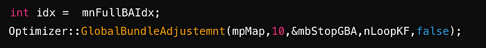
Performing the Optimization

The function records the current full bundle adjustment index and then calls the Optimizer::GlobalBundleAdjustemnt function. This function performs the global optimization on the map, taking in the map pointer (mpMap), a maximum of 10 iterations, a stop flag pointer (&mbStopGBA), the loop keyframe ID (nLoopKF), and a boolean flag indicating whether to use a robust kernel.

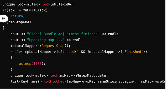
Updating Map Points and KeyFrames

After the optimization, the function checks if the current full bundle adjustment index matches the recorded index and if the bundle adjustment wasn’t stopped prematurely. If these conditions are met, it prints a message and requests the local mapper to stop. It waits until the local mapper has stopped or finished.

A lock on the map update mutex is acquired to ensure thread safety during the map update process. The function then initializes a list of keyframes to check, starting from the origin keyframes.

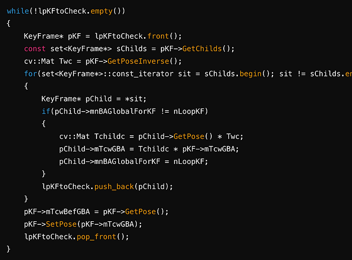
Propagating Corrections through the Spanning Tree

The function propagates the corrections through the spanning tree starting from the origin keyframes. For each keyframe, it updates the poses of its child keyframes using the optimized poses and the transformations. The poses of the keyframes are then updated to their optimized values.

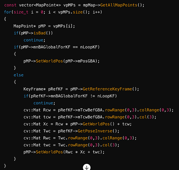
Correcting MapPoints

The function iterates through all the map points, updating their world positions. If a map point was optimized during the global bundle adjustment, its position is set directly. Otherwise, its position is updated according to the correction of its reference keyframe.

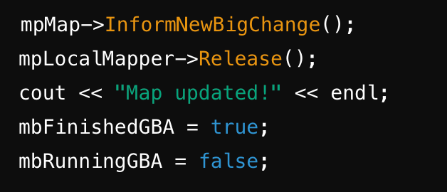
Finalize update

Finally, the function informs the map that a significant change has occurred, releases the local mapper, and prints a message indicating the map has been updated. It then sets the mbFinishedGBA and mbRunningGBA flags to true and false, respectively, to indicate the completion of the global bundle adjustment process.

ref: https://github.com/raulmur/ORB_SLAM2?tab=readme-ov-file

paper: https://github.com/raulmur/ORB_SLAM2?tab=readme-ov-file

youtube explanation: https://www.youtube.com/watch?v=z4ldKGh12ok