
Why we need quantization in edge computing?
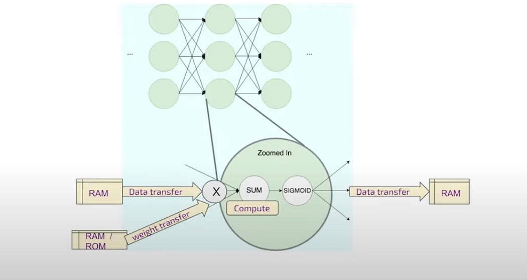
a neuron
The edges and nodes are computational operations and there are some mappings with the hardware. But when every edge eventually has some transfer of data and that needs some storage even if temporary and very close to memories. Hence, if there is low bit, there will be less transfers amount of transfer of data and less storage and less compute. Good for edge computing and low power consumption.
data transfer in nodes
Let’s understand from digital signal point of view:
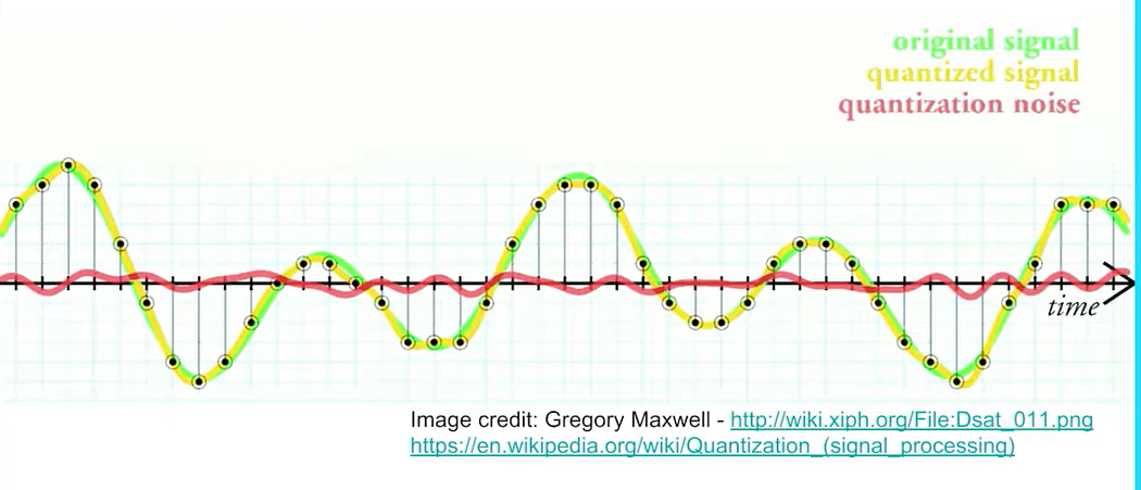
Digital signal

higher the bit smoother the curve and less noise
Here, with quantization, the noise will increase. In the image the green curve is much smoother with higher bits.
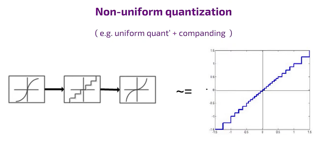
on-unifom like sigmoid
In case of quantization in non uniform fashion, the staircase is non uniform the steps are bigger in other parts.
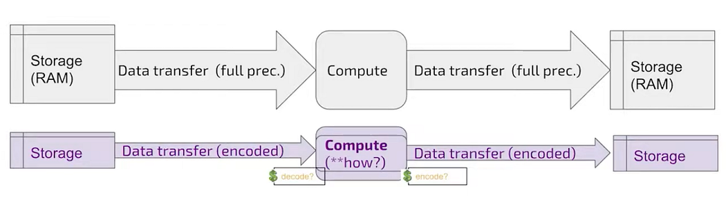
How to implement?
To pass the signal through time and nonlinear transformation then make uniform quantization and transform again. This method is sometimes referred to as compound compression and expansion, where the signal is compressed and then expanded, and vice versa.
Eventually the main conflict of the implementation is always between a dynamic range and the precision so when you make the named range large then your bins are larger and the precision is smaller and vice versa.
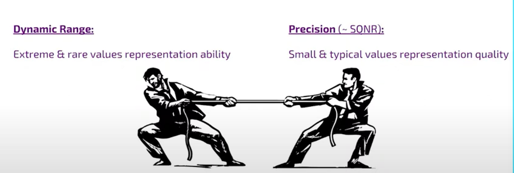
tussle between dynamic range and precision
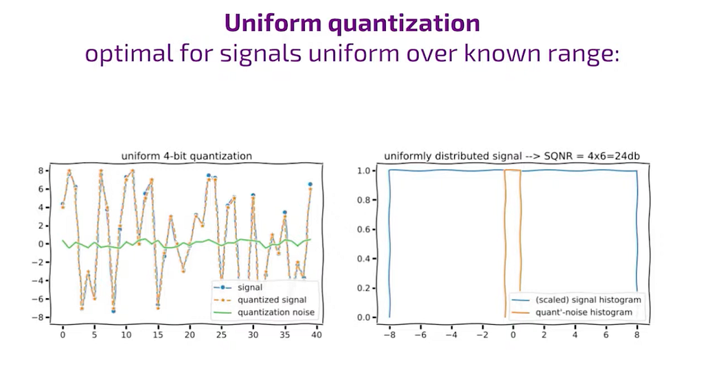
uniform signal
Uniform Signal
When the signal’s distribution is uniform within the range of -8 to 8, the quantization noise also follows a uniform distribution within plus and minus, say 5. This typically occurs when the step size is one, and the signal-to-noise ratio is relatively high. In this scenario, if we aim to quantize the signal to four bits (which is an ideal case), all the bins are equally utilized in the histogram, showcasing a uniform distribution of the signal across the range of -8 to 8.
A happy case:
When the step size is one and the signal-to-noise ratio is two to the power of a bit, everything looks wonderful.
Non-uniform signal
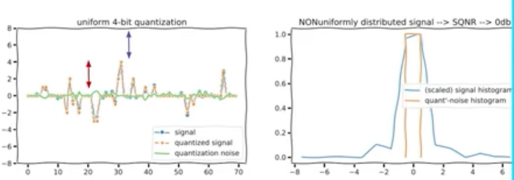
non-uniform signal
If our signal is non uniformly distributed then uniform quantization is not so optimal and the SQNR are the ratio of signal to noise magnitudes can go down even close to zero when most four.
Signals are typically within the order of magnitude of the quantization bin. For instance, muscle signals are often in the same order of magnitude as the noise. This means that as we increase the dynamic range, we tend to lose one bit of precision. This can lead to unexpected quantization results, such as quantizing to seven bits instead of the desired eight bits. These variations can be attributed to different factors, especially in the context of neural networks.
Consider an example where two channels require the same encoding due to technical constraints. One channel has a larger dynamic range represented by an orange signal, while the other channel’s signal is smaller and represented by a blue signal (diagram above). In quantization, sharing parameters between these channels can lead to precision loss for the smaller signal, as it doesn’t receive enough bits. This highlights that in quantization, the concept of “sharing is caring” doesn’t apply; rather, maintaining distinct boundaries ensures better precision.
The challenge arises from the gaps between the effective dynamic range of the signal and the range used for quantization. These gaps influence how the range is divided into bins, affecting the overall precision. This gap issue is common in neural networks, where the distributions of activations and weights exhibit non-linearity and non-uniformity.
Some more context:
In the context of digital signal processing and quantization, a 1-bit precision loss refers to the reduction in the number of bits used to represent the magnitude of a signal accurately. Each bit in a digital representation contributes to the overall precision of the signal measurement.
Bit Precision: In digital systems, the precision of a signal measurement is often quantified in terms of bits. For example, an 8-bit system can represent 2⁸ = 256 distinct levels or values. Each additional bit doubles the number of possible levels, increasing the precision.
Dynamic Range: The dynamic range refers to the difference between the smallest and largest values that can be represented or measured by a system. For instance, if a system has a dynamic range of 0 to 100 units, it can accurately measure values within that range.
Precision Loss Example: Imagine you have an 8-bit analog-to-digital converter (ADC) that measures voltages from 0 to 5 volts. With 8 bits, you can represent 2⁸ = 256 voltage levels, which means each level corresponds to approximately 5/256 = 0.0195 volts of precision.
Now, if you decide to increase the dynamic range of the ADC to measure voltages from 0 to 10 volts, the same 8 bits are used. However, with a wider range, each quantization level now represents 10/256 = 0.0391 volts. This doubling of the voltage range per level effectively reduces the precision by half. You’ve lost one bit of precision because the same number of bits now covers a larger range of values.
Hence, a 1-bit precision loss occurs when the dynamic range of a signal increases without a corresponding increase in the number of bits used for quantization. This reduction in precision can lead to less accurate representation and measurement of fine details or small changes in the signal, especially when the signal and noise levels are close or of similar magnitudes.

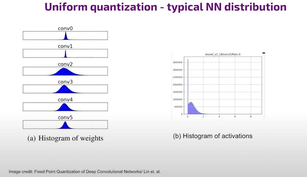
Quatization with respect to NN
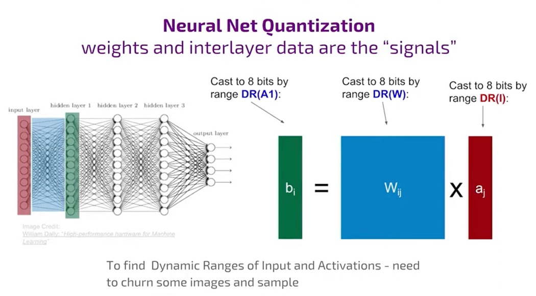
DR is dynamic range
For the weight, W, the dynamic range(DR) determination is relatively easy because the data is available.
Only problem is with the activation.
The range of values for activation is static and it’s not available upfront.
So, if you’ve just downloaded a pre-trained network from the internet, you’ll need to input some images, pass them through the network, compute the results, and then analyze the values obtained to determine the required range. This process is called casting.
NN
Activation needs asymmetric quantization. It is an asymmetric case of unsigned integer usually used for activations for the data that flows between layers.
casting
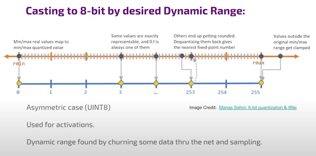
casting (image credit Manas Sahini)
Ideally, this approach works well for most signals but may not perform as well for very rare or irrelevant values. In such cases, unsigned integers are commonly used for activations, which represent the data flowing between layers in the network.
For instance, let’s say we’ve identified the range we prefer from the mean to the maximum value. Any values that needs to be quantized are rounded to the nearest bin edge, meaning the nearest whole number, and values outside this range are clamped. In this scenario, we clamp values that exceed the maximum.
For Weights, symmetric quantization,
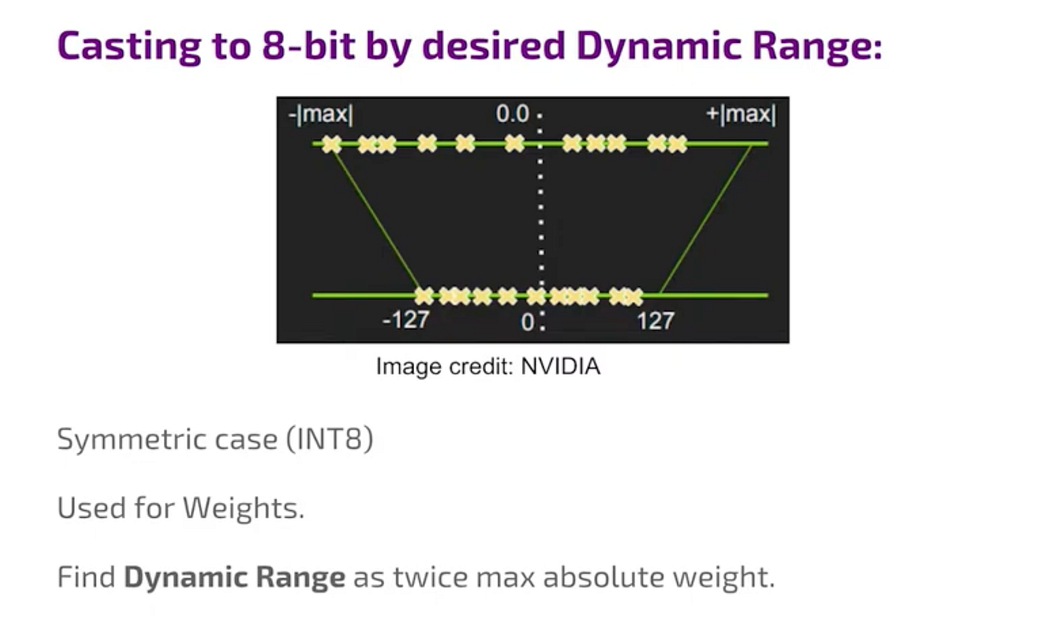
for weight
principle is exactly the same only difference in the symmetric case, i.e, the Weights case, finding the DR is easier — find the max weight and twice this value is the range that you want to quantize into those 255 values that 8-bit. (Why?) 2⁷ to 2⁸ (casting).

one layer CNN
This is a one layer CNN —there is data input and also we have the weight they are used to compute some intermediate representation and then nonlinear activation act on this and the output data is the same as input data for the next layer and then on all of these stages the two inputs the computation and the one output will replace the original high precision floating point 32-bit numbers by 8-bit quantized numbers. But is that all there in it? There are many details that are omitted here in this simple picture and there can be
Recoding
Blue color is sum of multiplications of 2 floating-point numbers and now you have sum of multiplication of two integer numbers (red ones) you need to somehow output a number which is quantized into a totally different possibly dynamic range which is optimal for this data flow and which this sum in red here. There are 2 things in play, the DR of the Weights and the static DR of the activation.
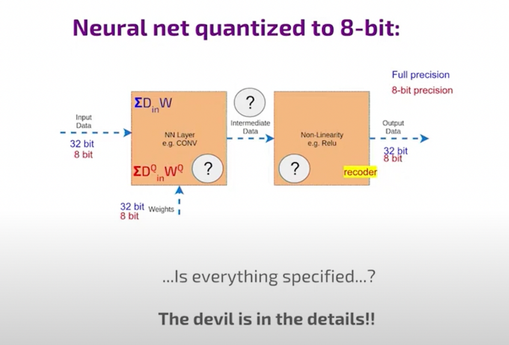
In the image there is an intermediate data and in the pipeline there are arithmetic in both sides of the hardware. On the Left hand side the Sum of multiplication of weight and input data and on the right hand side, i.e, the second part, it’s the non-linear function like Relu or Sigmoid. If it’s Relu, it’s relatively straightforward, you find the sign and zero it out. If it’s sigmoid, you compute it approximately. It’s a true for another genuinely nonlinear smooth function. This approximation involves a balance between precision and computational effort, leading to various details. The second part of the hardware takes care non-linearity and it also somehow recode to the next step so that one thing that everyone designing quantized implementation must implement somehow
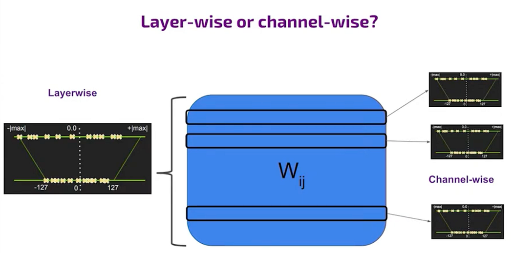
layer wise and channelwise quantization
Quantization can vary significantly depending on whether it’s channel-wise or layer-wise. Channel-wise quantization involves finding different dynamic ranges for each slice of the weight matrix related to an output channel, offering optimization benefits but with added complexity in control. Layer-wise quantization, however, determines one dynamic range for the entire weight matrix, simplifying control but limiting optimization. This additional degree of freedom in channel-wise quantization allows for more optimization, but it comes with a cost. Decoding the weights during computation requires knowing the specific channel, which can complicate control regardless of whether it’s a specialized processor or a general-purpose one.

Layer-wise quantization, commonly used, faces challenges due to the different dynamic ranges of channels. In comparison, channel-wise quantization involves taking the union of dynamic ranges across all channels, showcasing different approaches in handling quantization challenges and their impact on precision.
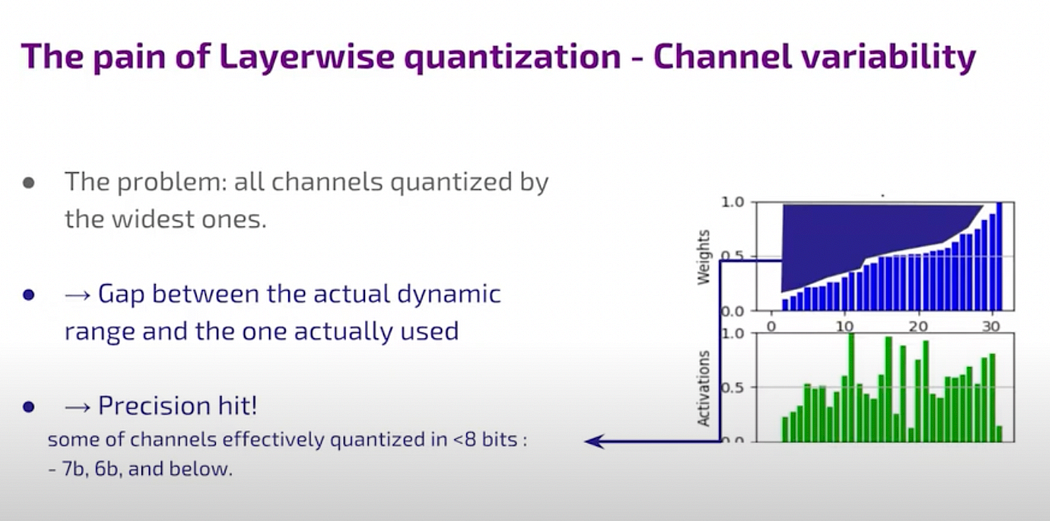
This disparity between the actual dynamic range needed and the one used for quantization creates a precision issue, potentially increasing noise compared to the signal. One approach to mitigate this is to amplify weaker channels and compress stronger ones to share the same range, optimizing quantization.
Optimization:
Simple quantization:
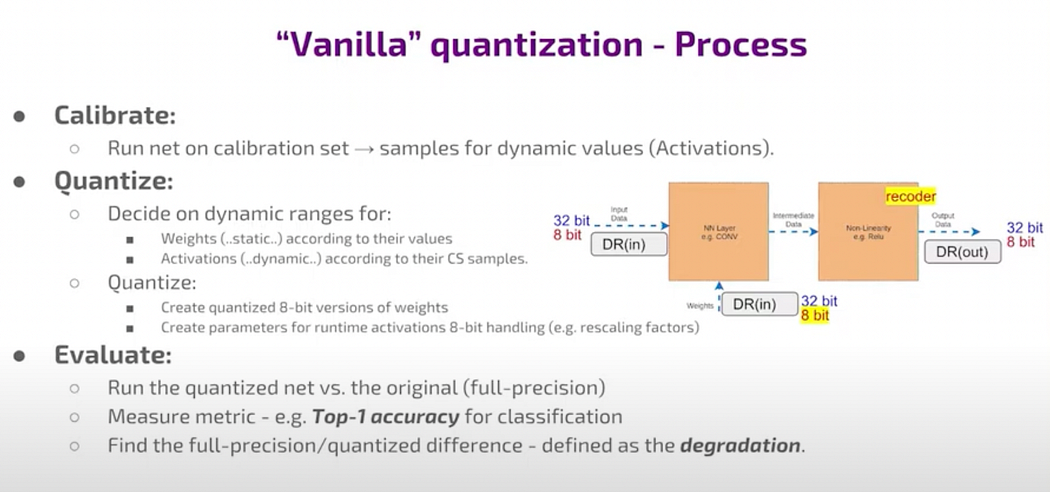
In the vanilla quantization process, you typically start by downloading a pre-trained network from the internet and aiming to run it on an 8-bit device. Calibration is necessary to quantize the activations, which involves sampling real data to determine statistical parameters to decide on the DR. For instance, you may decide on quantization thresholds based on maximum values or percentile thresholds (say 99 percentile), possibly sacrificing some high outliers. The output of this process includes quantized weights, usually in 8-bit format, indicated by the yellow outputs. Data cannot be quantized beforehand due to dynamic quantization nature, so you set parameters for the recoder that handles operating on recoded data efficiently. This recoding process maintains compression throughout the computation, leveraging linear transformations for uniform quantization, which simplifies the process while ensuring accuracy metrics like top one accuracy are met.

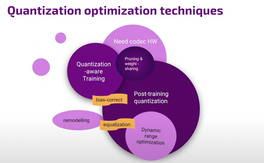
Here’s the main approach to optimizing quantization: there’s a divide between techniques requiring training quantization, which is the best option if you have the necessary resources, and post-training quantization. Post-training involves mathematical adjustments after training without retraining the model. This practical approach is common when resources for retraining are limited. Techniques like pruning and weight sharing fall under this category. Another set of methods involves specialized hardware due to non-linear encoding or sparsity requirements, which may necessitate decoding processes in software or hardware, incurring costs. You can also modify the network structure, like splitting layers or changing portions of layers, to optimize.
What does Hailo AI accelerator do?
Hailo’s channel equalization
One contribution is channel equalization, a post-training method focused on optimizing dynamic range differently from typical clipping methods.
When operations are linear, performing mathematics on encoded data is straightforward without the need for decoding. However, non-linear encoding or specialized encoding, such as pruning-induced sparsity, may require decoding processes, incurring computational costs in hardware or software. Alternatively, you can modify the network structure by splitting layers or changing portions of layers.
More on this how Hailo handles the quantization in another article.
